Fab Trade-Offs: Better Cycle Time for the Status Quo

By Jennifer Robinson

A goal in most wafer fabs is low, predictable cycle time. While there are structural conditions in fabs that make achieving this goal difficult (high product mix, reentrant flow, time constraints), there are also choices that fab teams make that drive up cycle times. It’s been my experience that fabs regularly trade better cycle time for three things: lower costs/higher revenue, higher yields, and what we’ll call the status quo (resistance to change).

We covered choices regarding cost and cycle time in Issue 26.04 and choices regarding cycle time and yield in Issue 26.05. In this article, we’ll discuss the third of these: changes that fabs could make that would likely reduce cycle time, but that require overcoming the powerful force of inertia. A sign of this resistance to change is hearing statements like:

• “But we’ve always done it this way.”
• “There’s no reason to make that change today.”
• “It’s what management wants. What can we do?”

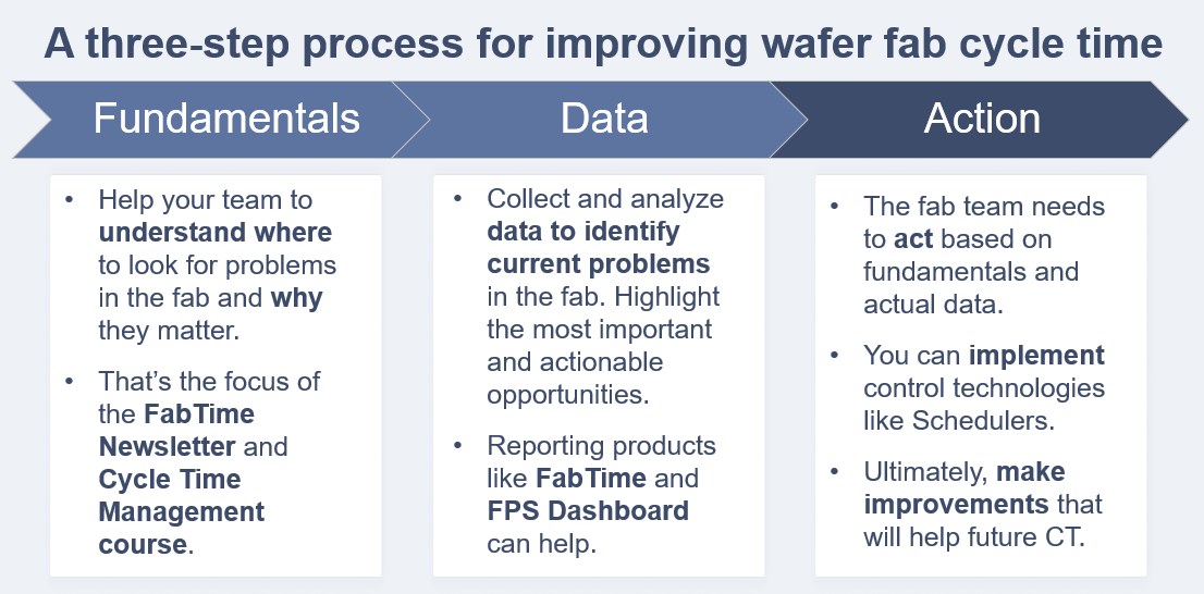
Back in Issue 26.01: Why and How Fabs Should Focus on CT Improvement, I proposed a three-step process for improving fab cycle time (shown below). After learning about the fundamentals and collecting data, I highlighted the need for the fab team to act. (You can read about a potential fourth step in this month’s Subscriber Discussion Forum.) The fact is, in fabs and in life, it’s not unusual to know that a change would be beneficial and still choose not to act. Or, at least, to choose not to act just yet. Below, we share some specific examples drawn from fabs. Our hope is that reviewing these may trigger a reassessment of the status quo for some fabs.

The easiest way to do something, on any given day, is to do it the same way you did it yesterday. Below, we review five operating practices that could, if changed, result in better wafer fab cycle time. We discuss the likely outcome of each vote for the status quo and suggest ideas for mitigating those impacts.

Of course, not all fabs do all these things. But I think most readers will find at least a few of these familiar. These are all behaviors that I’ve heard about over the years from people who work in fabs.

1. Group PMs and other unavailable periods: When a tool is down, there’s a natural tendency for the maintenance team to say: “Since this tool is down anyway, let’s also take care of this other required maintenance.”

• Likely outcome: Grouping PMs can be efficient in reducing the amount of required qualification time for the tool, and in the allocation of the maintenance team’s time. However, this practice is generally terrible for cycle time, especially for one-of-a-kind tools. The issue is that longer periods of unavailable time allow WIP bubbles to build up, resulting in higher queue times. This is described in detail in Issue 22.01: On Breaking Up PMs and Other Unavailable Periods.
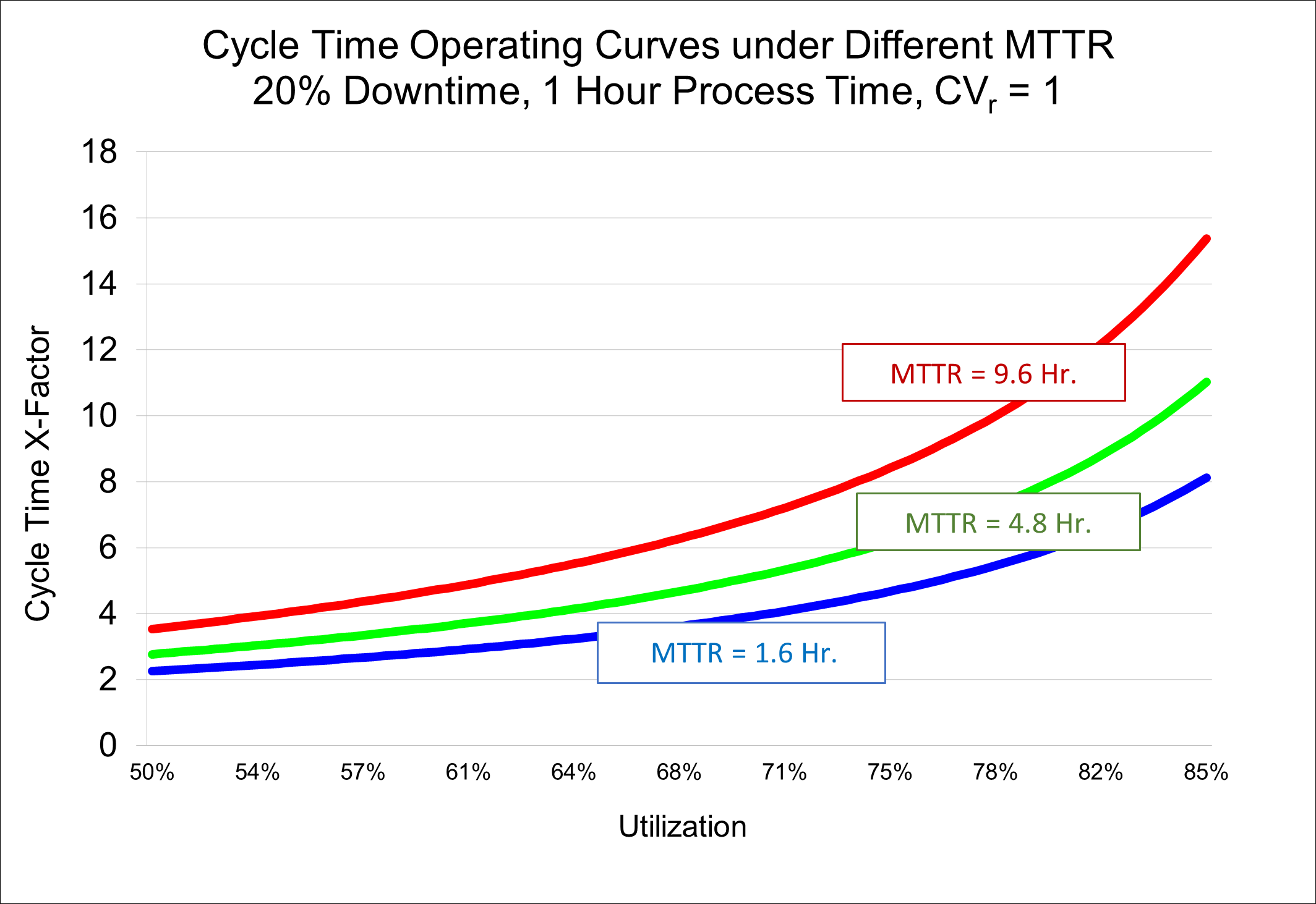
• As an illustration of this behavior, consider the operating curves below. In all cases, a one-of-a-kind tool is unavailable 20% of the time. On the blue curve the tool is taken down, on average, every 8 hours for 1.6 hours (20%). On the green curve, the tool is down once every 24 hours for 4.8 hours (still 20%). On the red curve, the tool is down once every 72 hours for 14.4 hours (still 20%). We can see that the x-factor is about twice as high for the red curve as it is for the blue curve. Even if, on the blue curve, the tool needs to spend some extra time doing quals, such that the utilization is a bit higher, it’s still much better to be on the blue curve than the red one. If you were to ask people from the manufacturing team with long experience whether they would prefer short, frequent interruptions or long, infrequent interruptions, they will almost always pick the short, frequent interruptions. This is because they’ve experienced the pain of fab disruption that comes from long downtime events.

• What you can do: The best way to keep this behavior from occurring is to move from tracking mean time between failures (MTBF) to tracking either mean time to repair (MTTR) or green-to-green time. (Green-to-green time is the total time elapsed between when the tool first becomes unavailable until it becomes available again, even if several scheduled and/or unscheduled downtime instances were logged in the interim. See Issue 25.04 or Issue 20.02 for details). Keeping the average duration of unavailable time low while continuing to monitor overall availability will help keep cycle times reasonable. Because this dynamic tends to be counter-intuitive for many people, this is an area in which cycle time training can be beneficial. See our cycle time class for more information.

2. Let operator preferences lead to one-of-a-kind tools: In fabs that give operators some degree of flexibility regarding which lot to run on which tool, we sometimes observe operator preferences for certain tools. This is called “soft dedication.” It can occur, for example, if one tool in a tool group is inconveniently located, or if a newer tool is preferred by the operators to the older version. (Or, I suppose, if the older tool is preferred to the newer version.)

• Likely outcome: Soft dedication leads to lower utilization levels on some tools, and higher utilization levels on others. This is typically a mismatch from what was expected in the fab’s capacity planning system. The tools with higher-than-expected utilization will have less buffer to protect against variability and hence will have higher cycle times.
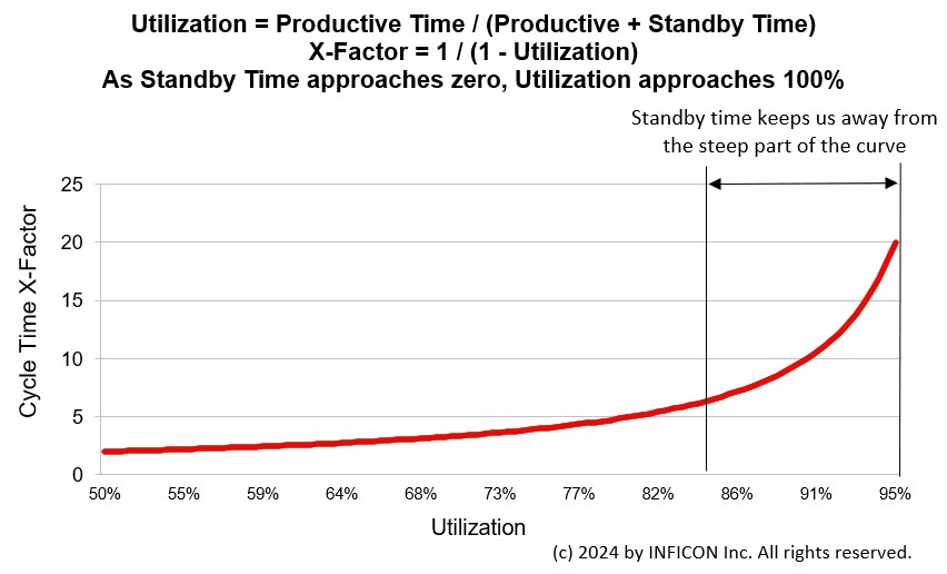
• The graph below shows the relationship between cycle time and utilization for a tool, and how standby time keeps the tool away from the steep part of the curve. Soft dedication reduces standby time for the tools that the operators prefer, resulting in higher cycle time per visit. The increase is nonlinear, so this is particularly an issue when it occurs on a tool that already has a relatively high utilization rate. For tool groups with considerable excess capacity, soft dedication is less of an issue.

• What you can do: Implementing a scheduler and requiring schedule compliance will drive down soft dedication. Highly automated and scheduled fabs don’t tend to see this issue.
• For fabs where operators have more leeway, we recommend checking to see if there are tool groups where soft dedication is contributing to high per-visit cycle times. You can do this by investigating tool groups that have high per-visit cycle times and comparing the moves per tool with availability efficiency. You’re looking for mismatches, where one or more tools has a lower move rate than would be predicted by the availability. High standby-WIP-waiting time on some tools in the tool group but not others can also be an indication of soft dedication, as the less favored tools sat idle even as WIP waited for the more favored tools to be available.

In the example below from the FabTime demo server, the chart on the left shows lower than expected moves (the black line) for Dev #1 compared to the other tools. The chart on the right shows higher than expected standby-WIP-waiting time for Dev #1.

• If you do find that soft dedication is increasing per visit cycle times, it makes sense to crack down on dispatch compliance in those areas. A mixture of education (about why we want similar utilization levels on all tools in a tool group) and data (showing how cycle time has increased because of the soft dedication in a particular area) can help drive change.

3. Put lots on hold for down tools: When a tool is expected to be unavailable for an extended period, some fabs will put lots requiring that tool on hold. The idea here is to let the operators know that there is nothing that needs to be done with those lots right now.

• Likely outcome: There are two problems with putting lots on hold for a down tool. First, the impact of the downtime on the lots’ cycle time is masked. This can make it harder for maintenance techs to know which tools are the top priority for repairs and make it harder to justify tool improvement projects or spare parts contracts down the road. Second, the fab might not have systems to automatically take the lots back off hold when the tool becomes available. This unnecessarily inflates lot cycle time.
• What you can do: The best thing is not to do this. Our recommendation is to not put lots on hold when the hold masks the reason for the lot’s delay. If you are going to do this, it’s important to use a specific hold code that allows for later analysis (e.g., “Hold for Down Tool”). The more detailed the better. It’s also very important to have some automated procedure for taking lots back off hold when the tool becomes available. At a minimum, you’ll want to make sure that the list of lots on hold is reviewed every shift, to identify any lots that may have mistakenly slipped through the cracks. Even with these precautions, you will still have the issue of not being able to see how much WIP is in queue for each down tool.

4. Leave tools idle during shift change: Many fabs assess operator performance based on number of moves completed per shift. When this is the case, there can be little incentive for operators to begin processing lots that will not finish by the end of the shift.

• Likely outcome: If operators leave tools idle with WIP waiting near the end of the shift, fabs will lose capacity on those tools. This lost capacity shows up as standby-WIP-waiting time on tool performance charts. Standby-WIP-waiting time pushes tools to a steeper place on the operating curve and drives up cycle time. See Issue 25.05 for more details.
• This behavior can sometimes be observed when looking at hourly trends in dynamic x-factor (DXF). DXF shows, at each point in time, the total WIP in the fab divided by non-rework WIP currently running on tools. Fabs that leave tools idle during shift change will see spikes in the DXF. The total WIP doesn’t change much from hour to hour, but the WIP running on tools can decrease sharply, spiking DXF. An example from a real fab is shown below. The fab’s hourly DXF normally floats between three and four, but spikes by more than 50% every 12 hours, at shift change.

• WIP hours. This is a newer metric developed by the FabTime user community to identify cycle time bottlenecks. WIP hours expands on tracking WIP by tool group by computing the estimated hours required to process the WIP that is in queue​. See Issue 20.03 for more details about WIP hours, and Issues 21.01, 21.03, and 21.04 for further discussion on short-term and cycle time bottlenecks. ​​

These metrics can give a forward look at cycle time:

• Dynamic x-factor, as defined above. When DXF is measured hourly and then averaged over time, it is equivalent to shipped lot x-factor. If it starts to drift upward, we get an early indication that shipped lot cycle time will (if the situation continues) increase in the future. See Issues 9.04 and 15.05 for more information about DXF.
• WIP turns and dynamic cycle time. WIP turns (moves per day divided by average WIP) give us an idea of the pace of the fab. If the turns rate is declining, we know that future cycle time will increase. The dynamic cycle time metric in FabTime adds the required number of steps for each lot to convert this pace into a future cycle time estimate in days. See Issue 24.03: Forward-Looking Cycle Time Metrics for more details.

Adding these cycle time-focused metrics can help your fab to identify improvement opportunities on a short-term and long-term basis and inspire people on your team to make necessary changes.

Trade-offs can be found in all aspects of life, and certainly in the complex environment of a wafer fab. Trade-offs between cycle time and cost and between cycle time and yield are actively managed. People decide about whether to spend money on tools, staff, or software in order to reduce cycle time. (See part one of this series.) They decide how much inspection and tool qualification is necessary for yield improvement, in some cases accepting higher cycle time in exchange for better yields. (See part two of this series.)

There’s a third type of trade-off that people make in managing fab cycle time that is a more passive choice. There are practices that could improve cycle time if they were changed, but that require overcoming the powerful force of the status quo. In this article we’ve highlighted five of these: grouping PMs, allowing soft dedication, putting lots on hold for down tools, allowing tools to be idle during shift change, and using metrics that do not account for cycle time. All of these, particularly the last two, can be influenced by careful selection of fab goals.

Does your fab do any of the things mentioned above? What else would you add to this list? What should we talk about next quarter? (Any responses shared will be shared anonymously.)

All past FabTime newsletters are available in PDF format from the FabTime Newsletter Archive. Please reach out to me for the link or look in the most recent email issue of the newsletter. You can download individual issues or download a zip file containing all past issues. Some articles have been re-published on the INFICON website. Those are linked above where mentioned.

For a more in-depth discussion of how these choices apply to your site, consider hosting a session of our four-hour web-based cycle time management course.

Further reading from this issue:

• Subscriber Discussion Forum
• Community Announcements page